Orbits, Access, And Coverage

This is the spatial foundation of an Astraeus study. It answers four related questions:

• where are the satellites over time?
• where are they relative to the rotating Earth?
• when can they see a ground site?
• how much of a selected area has one or more satellites in view?

flowchart LR ORBIT["Constellation and orbit"] --> PROP["SGP4 propagation in TEME"] PROP --> EARTH["Earth-fixed WGS-84 geometry"] EARTH --> ACCESS["Ground-site access"] EARTH --> COVERAGE["Point and area coverage"]

Ground access and coverage are separate analyses over the same propagated timeline. Requesting either stage automatically includes its required upstream work.

Propagation Model

Astraeus currently uses SGP4 for propagation. simulation.propagator accepts auto or sgp4; auto resolves to the same supported SGP4 implementation. The output is sampled at simulation.step_s from the requested UTC start time over the requested duration.

Common constellation authoring options are:

Design	Use it for
Walker	regularly phased circular or near-circular shells
Streets of Coverage	deriving a circular constellation from a geometric coverage target
Explicit planes	directly specifying plane RAAN, phasing, and satellite counts
Multiple shells	combining independently defined designs in one constellation

Orbit definitions support circular_altitude and general keplerian elements. The latter enables eccentric near-Earth cases such as Molniya-style studies within the supported SGP4 regime.

The primary propagation artifacts are:

Artifact	Contents
states/timeline_state_vectors_teme.parquet	position and velocity for every timestamp and satellite
states/timeline_summary.json	frame, dimensions, cadence, and backend metadata
states/satellites.json	resolved satellite inventory
config/resolved_constellation_layout.json	synthesized shells, planes, slots, and identities

Reference Frames

Propagated states are stored in TEME. Ground geometry converts those states to WGS-84-aligned ITRS/ECEF coordinates, then into the local east-north-up frame of each ground site or grid point.

flowchart LR TEME["TEME state"] --> ROT["Earth rotation and polar motion"] ROT --> ECEF["ITRS / ECEF"] SITE["WGS-84 latitude, longitude, altitude"] --> ENU["Local ENU frame"] ECEF --> ENU ENU --> OBS["Range, elevation, azimuth, visibility"]

The terrestrial transform uses bundled offline IERS Earth-orientation data. Dates outside its supported range produce a warning and use the documented degraded transform rather than silently fetching changing external data.

Ground-Site Access

Use the ground_access stage when the question is whether and when satellites can see named sites. Each site defines geodetic latitude, longitude, altitude, and its own minimum elevation mask:

ground:
  sites:
    - site_id: MADRID
      latitude_deg: 40.4168
      longitude_deg: -3.7038
      altitude_m: 650.0
      min_elevation_deg: 10.0

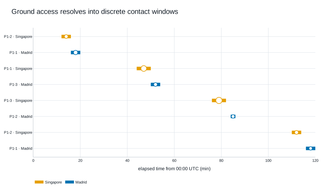
Each sampled satellite/site pair reports range, elevation, azimuth, line-of-sight, and access state. Azimuth is clockwise from true north in [0, 360) and is blank at exact numerical zenith.

Access windows are derived from the simulation samples. Window boundaries, maximum elevation, and minimum range are therefore sampled timestamps rather than interpolated event roots. Use a finer simulation.step_s when short passes or pass timing need more resolution.

Geographic Coverage

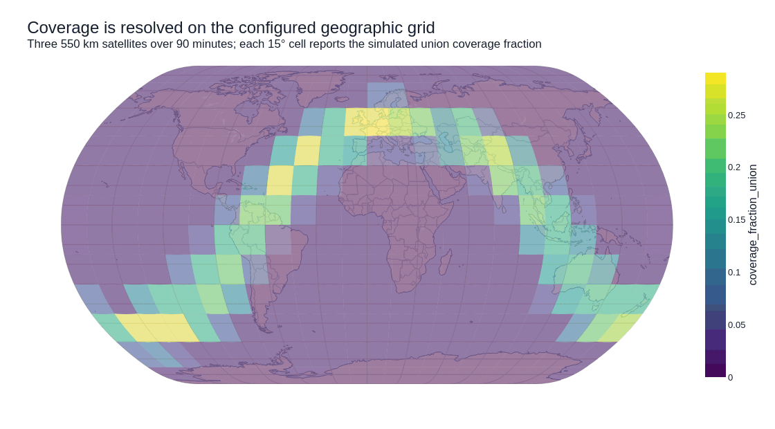
Use the coverage stage for visibility over a regular latitude/longitude grid or selected areas. A compact regional definition looks like this:

geography:
  coverage_scope: roi_only
  selection: europe
  grid_step_deg: 2.5
  min_elevation_deg: 20.0
  coverage_folds: [1, 2]
  areas:
    - area_id: europe
      kind: polygon
      polygon:
        - {lat_deg: 35.0, lon_deg: -10.0}
        - {lat_deg: 35.0, lon_deg: 30.0}
        - {lat_deg: 60.0, lon_deg: 30.0}
        - {lat_deg: 60.0, lon_deg: -10.0}

coverage_scope: global evaluates the global grid and can still tag configured areas. roi_only evaluates only grid centers selected by the configured area geometry. Areas may be explicit bounding boxes or polygons, or reusable built-in land, ocean, continent, belt, hemisphere, and polar presets.

Coverage Folds

A fold of N is satisfied when at least N selected satellites are visible at the same sample. Fold 1 is ordinary union coverage. Requested folds are sorted and deduplicated, fold 1 is always included, and an unattainable fold produces an explicit zero result rather than an error.

Geometric coverage resolves visibility on the selected grid. RF link budget, capacity, scheduling, routing, demand, and service delivery are resolved by downstream mission and communications analyses.

Equal-Point And Surface-Weighted Results

Astraeus reports both aggregation modes because they answer different questions:

Result	Interpretation
Equal-point mean	Every selected grid point has equal influence. Useful for comparing the sampled points themselves.
Surface-weighted mean	Each point is weighted by the spherical solid angle of its represented cell. Use this as the primary geographic-area result.

Equal-point aggregation can over-represent high-latitude rows on a regular latitude/longitude grid. Existing coverage_fraction_union_mean fields retain their historical equal-point meaning; the explicit coverage_fraction_union_point_mean and coverage_fraction_union_area_weighted_mean fields remove ambiguity.

Polygon membership is determined using the grid-cell center. Selected boundary cells retain their full represented spherical weight. Reduce grid_step_deg when that boundary approximation matters.

Main Outputs

Artifact	What it answers
geometry/access_samples.*	What were range, elevation, azimuth, and access at each sample?
geometry/access_windows.*	When did each sampled pass begin and end, and what were its extrema?
geometry/geometry_summary.json	Which conventions, shapes, and sampling policies were used?
coverage/coverage_summary.json	What are the global point and surface-weighted results and resolved folds?
coverage/coverage_summary_points.*	What were union coverage, revisit, and visible-satellite counts by point?
coverage/coverage_summary_*_by_fold.*	How did point, area, and global results change by fold?
coverage/coverage_summary_by_area.*	What were the fold-1 equal-point and surface-weighted area results?
coverage/coverage_points.*	Which points and represented cell weights were evaluated?
coverage/coverage_gap_hist_by_point.*	What revisit-gap distributions occurred by point?

Per-sample coverage tables can become very large. They are emitted only when artifacts.write_coverage_raw_samples is enabled; summaries are sufficient for most studies.

Packaged Examples

After copying the installed resources, use:

Question	Example
Propagate a compact constellation	astraeus-resources/examples/user/first-orbit.yaml
Inspect ground-station passes	astraeus-resources/examples/user/ground-access.yaml
Compare point and area-weighted regional coverage	astraeus-resources/examples/user/regional-coverage.yaml
Exercise first-shell-scale global coverage	astraeus-resources/examples/user/large-leo-global-coverage.yaml

The last entry is a batch with three 1,584-satellite, 24-hour cases and is meant as a deliberate large-scale exercise rather than a quickstart.

Interpretation Limits

• Propagation, access, and coverage share the configured time cadence; a coarse cadence can miss short events and under-resolve revisit gaps.
• SGP4 results inherit the validity limits of their generated or supplied mean element representation.
• Coverage reports sampled geometric visibility. Operational availability requires the relevant downstream service and communications analysis.
• Geometry uses the declared ellipsoid, elevation masks, and sampled cadence; terrain, atmospheric refraction, obstruction masks, and continuous-time event refinement remain outside this calculation.
• Finer geographic grids increase runtime and artifact volume quickly.

For exact RunSpec fields, see the RunSpec reference. For scientific evidence and acceptance bounds, see Scientific validation.